1 Introduction
what is machine learning
supervised learning
- supervised learning
- regression problem
- predict a continuous valued output
- classification problem
- predict a discrete valued output
- regression problem
SVM(Support Vector Machine) is a kind of generalized linear classification that classifies data by supervised learning
unsupervised learning
-
unsupervised learning
- Cluster Algorithm
- Google news
- Facebook friends
- Cluster Algorithm
2. Linear Regression with One Variable
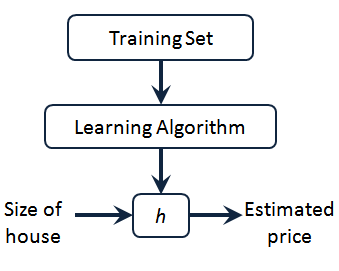
2.1 Model Representation
Linear regression with one variable.
Univariate linear regression.
m —— the number of training examples
x —— input
y —— output
h —— hypothesis function
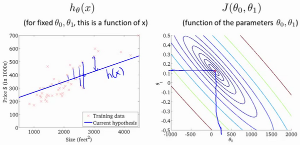
$h_\theta \left( x \right)=\theta_{0}+\theta_{1}x$
2.2 Cost function
also called square error function or square error cost function.
help figure out how to fit the best possible straight line to our data.
how to choose parameter values to make hypothesis function fit better.($J \left( \theta_0, \theta_1 \right) = \frac{1}{2m}\sum\limits_{i=1}^m \left( h_{\theta}(x ^{(i)})-y ^{(i)} \right)^{2}$)
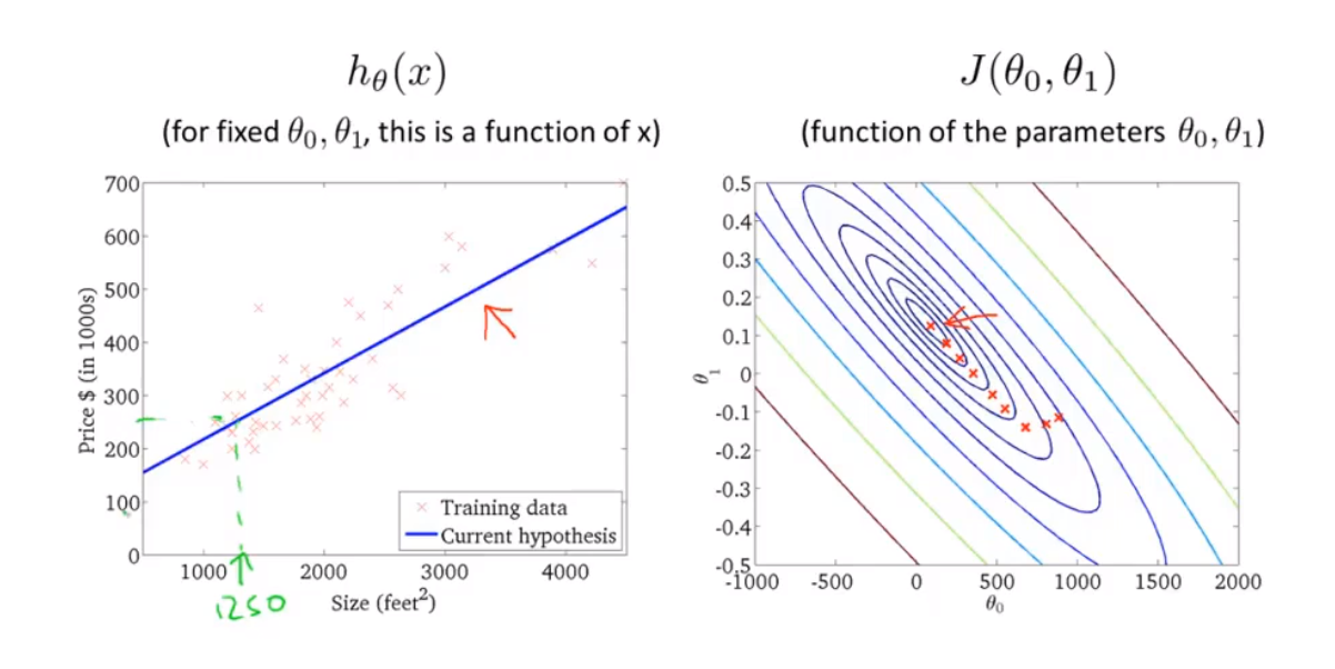
2.3 Cost Function - Intuition 1
For each value of theta one corresponds to a different hypothesis or to a different straight line fit. And for each value of theta one, we could then derive a different value of J of theta one. And value of J of theta one plot the picture on the right.
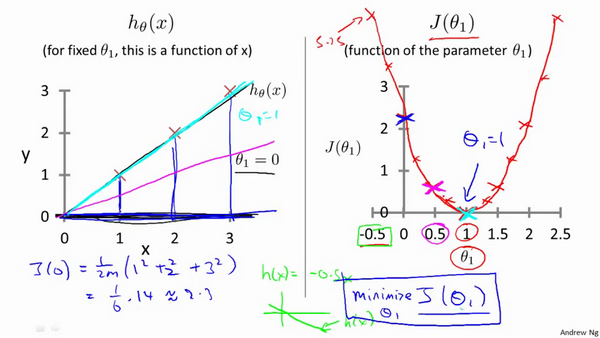
The optimization objective for our learning algorithm is we want choose the value of theta one that minimizes J of theta one. This was our objective function for the linear regression.
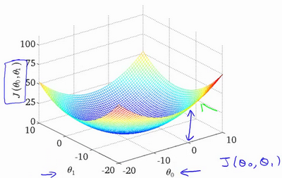
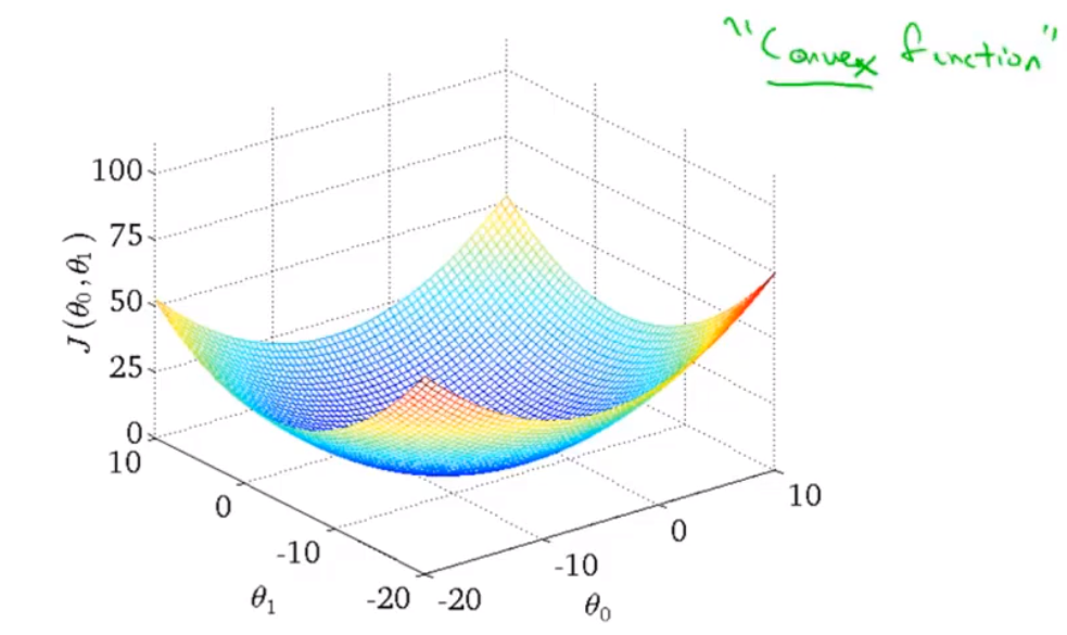
2.4 Cost Function - Intuition 2
1 parameter 2-D plot
2 parameters 3-D plot
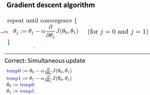
2.5 Gradient Descent
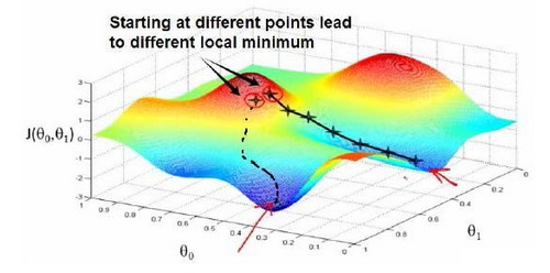
Imagine that this figure shows a hill, you are physically standing at a point one the hill. Gradient descent is to spin 360 degrees around and ask “if I were to take a little baby step in some direction, and I want go downhill as quickly as possible, what direction do I take?”
Go until you converge to a local minimum. If you start at different point, gradient descent will take you to the second local optimum.
This is batch gradient descent algorithm and $\alpha$ refer to the learning rate. We need update the $\theta_0$ and $\theta_1$ simultaneously.
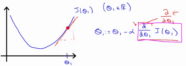
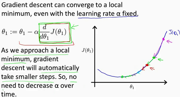
2.6 Gradient Descent Intuition
For single variable function, partial derivative equal to derivative.
The direction of the derivative is opposite to the direction to be changed, so $\alpha$ is preceded by a minus sign. Sign of partial derivative refer to the direction you need to go and $\alpha$ refer to the length of your every little step. If $\alpha$ is too small, gradient descent can be slow. If $\alpha$ is too large, gradient descent can overshoot the minimum. It may fail to converge, or even diverge.
The reason why we don’t need to decrease $\alpha$. (automatically take smaller steps)
2.7 Gradient Descent For Linear Regression
Apply gradient descent to minimum our squared error cost function.
Partial derivative of cost function for linear regression:
$\frac{\partial }{\partial \theta_j}J(\theta_0,\theta_1)=\frac{\partial }{\partial \theta_j}\frac{1}{2m}\sum\limits_{i=1}^m \left( h_{\theta}(x ^{(i)})-y ^{(i)} \right)^{2}$
$j=0$ : $\frac{\partial }{\partial \theta_0}J(\theta_0,\theta_1)=\frac{1}{m}\sum\limits_{i=1}^m \left( h_{\theta}(x ^{(i)})-y ^{(i)} \right)$
$j=1$ : $\frac{\partial }{\partial \theta_1}J(\theta_0,\theta_1)=\frac{1}{m}\sum\limits_{i=1}^m \left( \left( h_{\theta}(x ^{(i)})-y ^{(i)} \right)\cdot {x^{(i)}} \right)$
Cost function for linear regression is always going to be a bowl-shaped function(convex function), it doesn’t have any local optima except for the one global optimum.
“Batch”: each step of gradient descent uses all the training examples.
3. Linear Algebra Review
3.1 Matrices and Vectors
vector is a matrix that has only one column.
3.2 Addition and Scalar Multiplication
add or multiply every element
3.3 Matrix Vector Multiplication
$m×n$ matrix times $n×1$ vector equal to $m×1$ vector
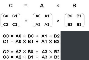
3.4 Matrix Matrix Multiplication
3.5 Matrix Multiplication Properties
all matrix:
$A×B≠B×A$(commutative property of multiplication)
$A×(B×C)=(A×B)×C$(associative property of multiplication)
Identity matrix:
identity matrix has ones along the diagonals and zero everywhere else.
$$\begin{bmatrix} 0 & -1 \\ 1 & 0 \end{bmatrix}$$
$AA ^{-1}=A ^{-1}A=I$
$AI=IA=A$
3.6 Inverse and Transpose
inverse of matrix($A^{-1}$)
only square matrices have inverses.
$AA ^{-1}=A ^{-1}A=I$
transpose:
let A be an m x n matrix, let $B = A^T$.
Then B is an n x m matrix and $B_{ij} = A_{ji}$.
$$\begin{bmatrix} 1 & 2 & 0 \\ 3 & 5 & 9 \end{bmatrix} = \begin{bmatrix} 1 & 3 \\ 2 & 5 \\ 0 & 9 \end{bmatrix}$$
4. Linear Regression with Multiple Variables
4.1 Multiple Features
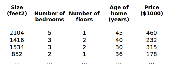
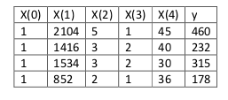
$\left( x_1,x_2,…,x_n \right)$ stand for multiple variables
$x^{(i)}$ is a vector and it stand for the $i^{th}$ training example
$x^{(2)}=\begin{bmatrix} 1416 \\ 3 \\ 2 \\ 40 \end{bmatrix}$
$x_j^{(i)}$ stand for the value $j$ in $i^{th}$ training example.
$x_2 ^{(2)}=3,x_3 ^{(2)}=2$
the form of the hypothesis:
$h_\theta \left( x \right)=\theta_0+\theta_1x_1+\theta_2x_2+…+\theta_nx_n$
For convenience of notation, we define $x_0$ to be equals one.
Now, $X$ is a $n+1$ dimensional feature vector; parameters $\theta$ is also a $n+1$ dimensional vector.
$X = \begin{bmatrix} x_0 \\ x_1 \\ x_2 \\ … \\ x_n \end{bmatrix} \theta = \begin{bmatrix} \theta_0 \\ \theta_1 \\ \theta_2 \\ … \\ \theta_n \end{bmatrix} \theta^T = \begin{bmatrix} \theta_0 \ \theta_1 \ \theta_2 \ … \ \theta_n \end{bmatrix}$
$h_\theta \left( x \right)=\theta_0 x_0 + \theta_1 x_1 + \theta_2 x_2+ … + \theta_n x_n$
$h_\theta \left( x \right)=\theta^TX$
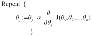
4.2 Gradient Descent for Multiple Variables
Gradient descent algorithm:
$J({\theta_0},{\theta_1}…{\theta_n})=\frac{1}{2m}\sum\limits_{i=1}^m{( h_\theta(x^{(i)})-y^{(i)})^2}$
when $n>=1$:
${\theta_0}:=\theta_0-a\frac{1}{m}\sum\limits_{i=1} ^m{(h_\theta(x ^{(i)})-{y} ^{(i)})}x_0 ^{(i)}$
${\theta_1}:=\theta_1-a\frac{1}{m}\sum\limits_{i=1} ^m{(h_\theta(x ^{(i)})-{y} ^{(i)})}x_1 ^{(i)}$
${\theta_2}:=\theta_2-a\frac{1}{m}\sum\limits_{i=1} ^m{(h_\theta(x ^{(i)})-{y} ^{(i)})}x_2 ^{(i)}$
|
|
4.3 Gradient Descent in Practice I - Feature Scaling
Feature scaling:
If you make sure that the features are on a similar scale, then gradient descents can converge more quickly.
If $\theta_1$ is larger than $\theta_2$, the cost function will like picture on the left. And if you run gradient descent on this sort of cost function, your gradients may end up taking a long time and can oscillate back and forth and take a long time before it can finally find its way to the global minimum.
A useful thing to do is to scale the features. If $x_1, x_2$ like on the right, the contours may look more like circles, and if you run gradient descent on a cost function like this, then gradient descent (you can show mathematically) can find a much more direct path to global minimum rather than much more complicated trajectory.
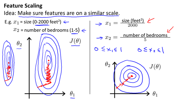
When we performing feature scaling, what we often to do is get every feature into approximately range $[-1,1]$ nether too small nor too large.
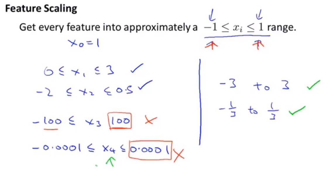
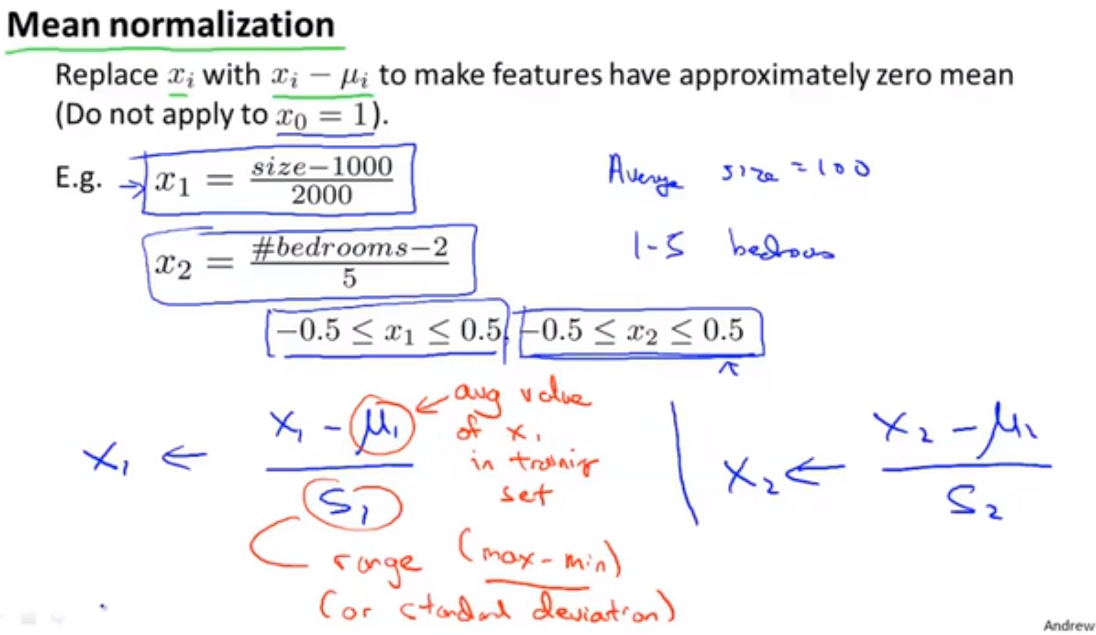
When performing feature scaling, sometimes people will also do what’s called mean normalization.
Place $x_i$ with $x_i-\mu_i$ to make feature have approximately zero mean.
More general rule: replace $x_1 <- \frac{(x_1-\mu_1)}{s_1}$, $\mu1$ is the average value of $x_1$ in the training sets, ans $s_1$ is the standard deviation of that feature. Then it will be roughly into these sorts of ranges.
4.4 Gradient Descent in Practice II - Learning Rate
See 2.6 Gradient Descent Intuition
$\alpha=0.01,0.03,0.1,0.3,1,3,10$
4.5 Features and Polynomial Regression
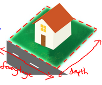
To predict the prize of the house we have two paras $h_\theta(x)=\theta_0+\theta_1\times{frontage}+\theta_2\times{depth}$
if we let $x=frontage * depth=area$ then $h_\theta(x)=\theta_0+\theta_1x$
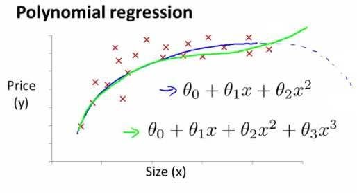
sometimes linear regression don’t fit all data, so maybe you want to fit a quadratic model like $h_\theta(x)=\theta_0+\theta_1x_1+\theta_2x_2^2$, it may be not fit well, then you can choose to use instead a cubic function line$h_\theta(x)=\theta_0+\theta_1x_1+\theta_2x_2 ^2+\theta_3x_3 ^3$
$h_\theta(x)=\theta_0+\theta_1(size)+\theta_2(size)^2$
$h_\theta(x)=\theta_0+\theta_1(size)+\theta_2\sqrt{size}$
polynomial regression fit a polynomial, like a quadratic function or a cubic function, to your data. Be aware that you have a choice in what features to use, and by designing different features you can fit more complex functions to your data than just fitting a straight line to the data, and in particular, you can fit polynomial functions as well.
PS: it is important to apply feature scaling if you are using gradient descent to get them into comparable ranges of values.
4.6 Normal Equation
Normal equation, which for some linear regression problems, will git us much better way to solve for the optimal value of the parameters theta.
So far the algorithm that we’ve been using for linear regression is gradient descent where in order to minimize the cost function $J of \theta$, we would take this iterative algorithm that takes many steps, multiple iterations of gradient descent to converge to the global minimum. In contrast, the normal equation will give us a method to solve for theta analytically, so that rather than needing to run this iterative algorithm, we can instead just solve for the optimal value for theta all at one go, so that in basically one step you get to the optimal value right there.
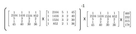
Set $\theta=(X ^TX) ^-1X ^Ty$, this will give you the value of $\theta$ that minimizes your cost function.
Normal equation don’t need feature scaling, thought it is important for linear regression.
CHOICES:
| Gradient descent | Normal equation |
|---|---|
| need to choose $\alpha$ | no need to choose $\alpha$ |
| need many iterations | don’t need to iterate |
| works well even when $n$ is large | need to compute$(X ^TX) ^{-1}$ |
| inverse O(n^3), slow if $n$ is very large |
4.7 Normal Equation Noninvertibility
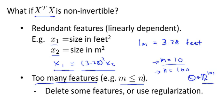
What if the matrix X transpose X is non-invertible? Some matrices do not have an inverse, we call those non-invertible matrices, singular or degenerate matrices. The issue or the problem of X transpose X being non-invertible should happen pretty rarely.
If X transpose X is non-invertible, there are usually two most common causes: The first cause is if somehow, in your learning problem, you have redundant features, concretely, if you try to predict housing prices and if $x_1$ is the size of house in square-feet and $x_2$ is the size of the house in square-meters(1 meter is equal to 3.28 feet), your two features are related via a linear equation, then matrix X transpose X will be non-invertible. Second thing that can cause it to be non-invertible is if you’re trying to run a learning algorithm with a lot of features. Concretely, if m is less than or equal to n.
5. Octave Tutorial
omitted
6. Logistic Regression
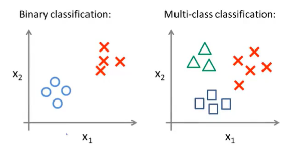
6.1 Classification
Logistic regression, actually a classification algorithm, has the property that the output the predictions of logistic regression are always between zero and one, and doesn’t become bigger than one or become less than zero.
6.2 Hypothesis Representation
Hypothesis representation, that is what is the function we’re going to use to represent our hypothesis when we have classification problem.
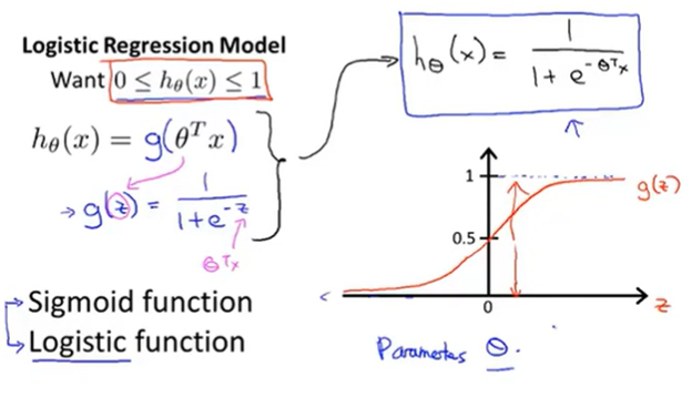
When we were using linear regression, $h_\theta(x)=\theta^Tx$ was the form of a hypothesis. For logistic regression, I’m going to modify this a little bit and make the hypothesis $h_\theta(x) = g(\theta^Tx)$, where g is $g(z)=\frac1{1+e^{-z} }$, this is called sigmoid function or logistic function(give rise to the name logistic regression)(Sigmoid function and logistic function are basically synonyms and mean the same thing. So the two terms are basically interchangeable).
$h_\theta(x) = \text{estimated probability that y=1 on input x}$
$h_\theta(x) = P(y=1|x;\theta)$ and $P(y=0|x;\theta)+P(y=1|x;\theta)=1$
6.3 Decision Boundary
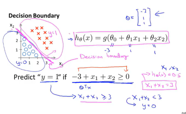
If $h_\theta(x)=g(\theta_0+\theta_1x_1+\theta_2x_2)$ and let $\theta=\begin{bmatrix} -3 \\ 1 \\1 \end{bmatrix}$
$x_1+x_2>=3$ is decision boundary.
|
|
6.4 Cost Function
J of $\theta$ ends up being a non-convex function if we are to define it as the squared cost function. We need to come up with a different cost function that is convex and so that we can apply a great algorithm like gradient descent and be guaranteed to find a global minimum.
Here’s a cost function that we’re going to use for logistic regression.
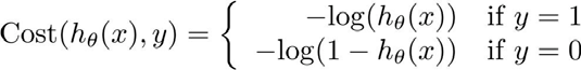
This function will penalize learning algorithm by a very large cost.

|
|
6.5 Simplified Cost Function and Gradient Descent
Cost function can be written in a simple one line: $cost(h_\theta(x),y)=-ylog(h_\theta(x))-(1-y)log(1-h_\theta(x))$
Then the cost function would be $J(\theta)=\frac1m\sum\limits_{i=1} ^mCost(h_\theta(x ^{(i)},y ^{(i)})=-\frac1m\sum\limits_{i=1} ^m[y ^{(i)}log(h_\theta(x ^{(i)}))+(1-y ^{(i)})log(1-h_\theta(x ^{(i)}))]$
This cost function can be derived from statistics using the principle of maximum likelihood estimation, which is convex and find parameters $\theta$ for different models efficiently.
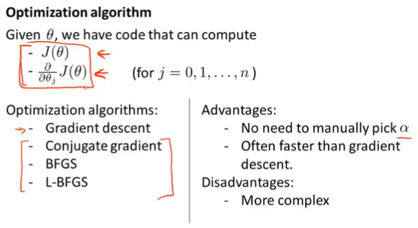
Given this function, in order to fit the parameters, what we’re going to do then is try to find the parameters $\theta$ that minimizes $j(\theta)$.${\underset\theta\min}j(\theta)$, this will give us a set of $\theta$. Finally if we’re given a new example with some et of features X. We can then take the thetas that we fit our training set and output our prediction as this $h_\theta(x)=\frac1{1+e ^{-\theta ^Tx}}$.
The way we are using to minimize the cost function is using gradient descent. If we want to minimize it as a function of $\theta$. Here’s our usual template for gradient descent, where we repeatedly update each parameter by updating it as itself minus a learning rate alpha times derivative term.
$$
\text{Want }min_\theta j(\theta):
\text{Repeat }
\theta_j:=\theta_j-\alpha\frac\partial{\partial \theta_j}j(\theta)
\text{ Simultaneous update all }\theta_j
$$
This algorithm looks identical to linear regression! So are they different algorithm or not? What have changed is $h_\theta(x)$, $h_\theta(x)=\theta^TX$ in linear regression and $h_\theta(x)=\frac1{1+e ^{-\theta ^Tx}}$ in logistic function. So even though the update rule looks cosmetically identical, because the definition of the hypothesis has changed, this is actually not the same thing as gradient descent for linear regression.
Feature scaling can help gradient descent converge faster for linear regression. The idea of feature scaling also applies to gradient descent for logistic regression.
6.6 Advanced Optimization
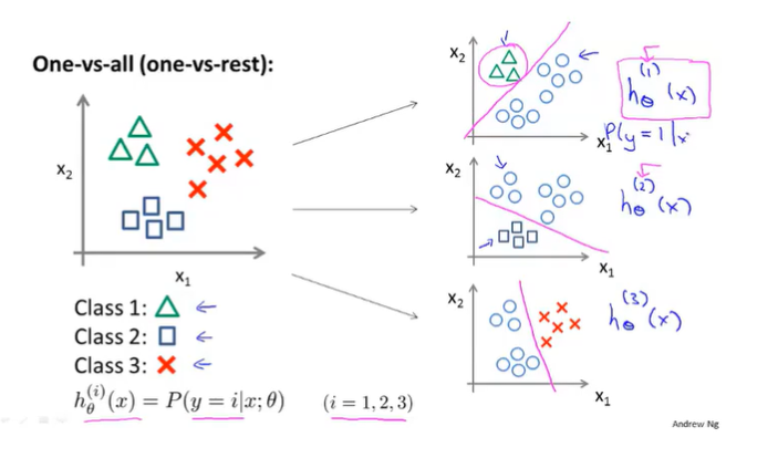
6.7 Multi-class Classification_ One-vs-all
Turn training set into three separate binary classification problems.
7. Regularization
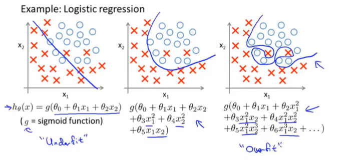
7.1 The Problem of Overfitting
When you apply algorithm to certain ML applications, thry can run into a problem called overfitting, that can cause them to perform very poorly.
Try too hard to fit the training set, so that it even fails to generalize to new examples.
Here is an instance of overfitting, and og a hypothesis having high variance and not really, and being unlikely to generalize well to new examples.
Debugging and diagnosing
recognize when overfitting and also when underfitting may be occurring.
Options:
-
- Reduce number of features.
- Manually select which features keep.
- Model selection algorithm.
Throwing away some features also throwing away some information.
-
- Regularization
- Keep all the features, but reduce magnitude/values of parameters$\theta_j$.
- Works well when we have a lot of features, each of which contributes a bit to predicting y.
7.2 Cost Function
The idea of regularization is if we have small values for the parameters, it usually correspond to having a simpler hypothesis.
In example, we penalize just $\theta_3 \text{ and }\theta_4$, make $\theta_3 \text{ and }\theta_4$ small and gave us a simpler hypothesis.
It is hard to pick in advance which are the ones that are less likely to be relevant. So in regularization, what we are going to do is take our cost function, and modify the cost function to shrink all of my parameters.
$J(\theta)=\frac1{2m}[\sum\limits_{i=1} ^m{(h_\theta(x ^{(i)})-y ^{(i)})} ^2+\lambda \sum\limits_{j=1} ^n{\theta_j ^2}]$
$\lambda$ is called regularization parameter. And what lambda does, is controls a trade off between two different goals. The first goal is captured by the first term of the objective, is that we would like to fit the training set well. And the second goal is we want to keep the parameters small, and that’s captured by the second term, by the regularization objective, and by regularization term.
What $\lambda$ does is the controls the trade off between the goal of fitting the training set well and the goal of keeping the parameter small, and therefore keeping the hypothesis relatively simple to avoid overfitting.
7.3 Regularized Linear Regression
Gradient descent:
In regularization, we penalize the parameters $\theta_1\theta_2$ and so on up to $\theta_n$, but we don’t penalize $\theta_0$, so when we modify this algorithm for regularized linear regression, we’re going to end up treating $\theta_0$ slightly differently.
Repeat until convergence{
$\theta_0:={\theta_0}-a\frac1m\sum\limits_{i=1} ^m((h_\theta(x ^{(i)})-y ^{(i)})x_0 ^{(i)})$
$\theta_j:=\theta_j-a[\frac1m\sum\limits_{i=1} ^m(h_\theta(x ^{(i)})-y ^{(i)})x_j ^{(i)}+\frac\lambda m\theta_j]$
$for$ $j=1,2,…n$
}
If you group all the terms together that depending on $\theta_j$, you can show that this update can be written equivalently as follows.
$\theta_j:=\theta_j(1-a\frac\lambda m)-a\frac1m\sum\limits_{i=1} ^m({h_\theta}(x ^{(i)})-y ^{(i)})x_j ^{(i)}$
Since $\alpha$ is small and m is big, so $(1-\alpha\frac\lambda m)$ is a number that a little bit less than one. That mean we’re shrinking the parameter a little bit, and then we’re performing similar update as before. Mathematically, what it’s doing is exactly gradient descent on the cost function $j \text{ of } \theta$ that uses the regularization term.
Normal equation:
If you are using regularization, then this formula would add a matrix inside.
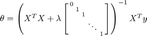
This new formula for $\theta$ is one that will give you the global minimum of $j$ of $\theta$.
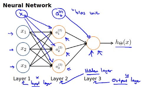
non-invertibility:
If you have fewer examples than feature, then this matrix X transpose X will be non-invertible, or singular(degenerate).
So long as the regularization parameter $\lambda$ >0, it is actually possible to prove that this matrix X transpose X plus parameter times this funny matrix will not be singular.
7.4 Regularized Logistic Regression
$J(\theta)=\frac1m\sum\limits_{i=1} ^m[-y ^{(i)}\log( h_\theta(x ^{(i)}))-(1-y ^{(i)})\log(1-h_\theta( x ^{(i)}) )]+\frac{\lambda }{2m}\sum\limits_{j=1} ^n\theta_j ^2$
|
|
Repeat until convergence{
$\theta_0:=\theta_0-a\frac1m\sum\limits_{i=1} ^m((h_\theta(x ^{(i)})-y ^{(i)})x_0 ^{(i)})$
$\theta_j:=\theta_j-a[\frac1m\sum\limits_{i=1} ^m(h_\theta(x ^{(i)})-y ^{(i)})x_j ^{(i)}+\frac{\lambda }{m}\theta_j]$
$for$ $j=1,2,…n$
}
This cosmetically looks identical to what we had for linear regression. But of course is not the same algorithm as we had, because now the hypothesis is defined using $h_\theta(x)=\frac1{1+e ^{-\theta ^Tx}}$.
8. Neural Networks: Representation
8.1 Non-linear Hypotheses
If we were try to learn a nonlinear hypothesis by including all the quadratic features, it was too large to be reasonable. So simple logistic regression together with adding in maybe the quadratic or the cubic features that’s just not a good way to learn complex nonlinear hypotheses when n is large, because you just end up with too many features.
Neural network turns out to be a much better way to learn complex nonlinear hypotheses, even when your input feature space, even when n is large.
8.2 Neurons and the Brain
omitted
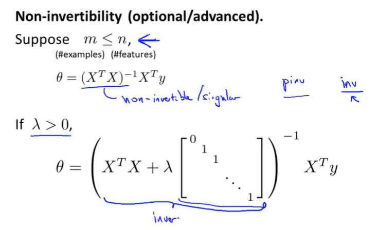
8.3 Model Representation I
8.4 Model Representation II
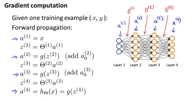
Forward propagation: Vectorized implementation
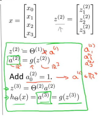
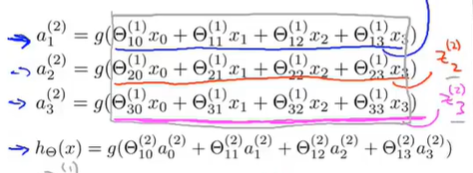
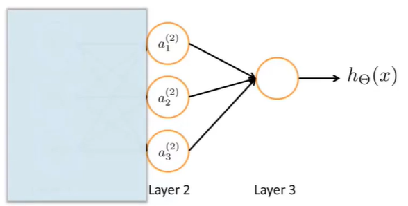
The right part of the picture looks a lot like logistic regression where what we’re doing is we’re using last node, that’s just the logistic regression unit and we’re using that to make a prediction h of x. The output $h_\Theta(x)=g(\Theta_0 ^{(2)}a_0 ^{(2)}+\Theta_1 ^{(2)}a_1 ^{(2)}+\Theta_2 ^{(2)}a_2 ^{(2)}+\Theta_3 ^{(2)}a_3 ^{(2)})$. $a_0,a_1,a_2,a_3$ are given by three given units. This is awfully like the standard logistic regression model. But where the features fed into logistic regression are these values computed by the hidden layer. Concretely, the function mapping from layer 1 to layer 2, that is determined by some other set of parameters, theta 1.
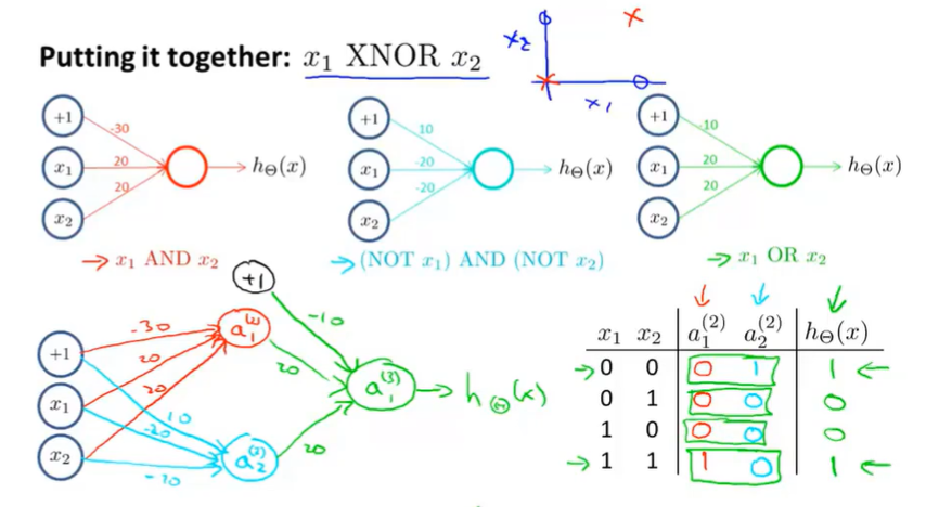
8.5 Examples and Intuitions I
Neural networks can be used to learn complex nonlinear hypotheses.
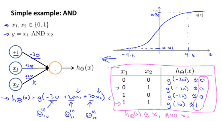
AND function:
OR function:
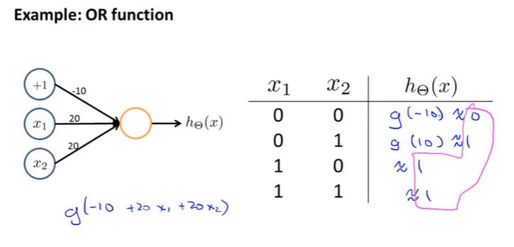
By taking different set of $\theta$, a single neurons in a neural network can be used to compute logical function.
8.6 Examples and Intuitions II
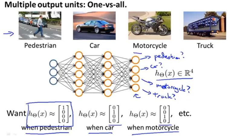
8.7 Multiclass Classification
We have 4 logistic regression classifiers, each of which is trying to recognize one of the four classes that we want to distinguish amongst.
9. Neural Networks: Learning
9.1 Cost Function
The cost function we use for the neural network is going to be a generalization of the one that we use for logistic regression.
Logistic regression:
$J(\theta)=-\frac1m[\sum_\limits{i=1} ^{m}y ^{(i)}\log h_\theta(x ^{(i)})+(1-y ^{(i)})log(1-h_\theta(x ^{(i)}))]+\frac\lambda {2m}\sum_\limits{j=1} ^n\theta_j ^2$
Neural network now outputs vectors in $R_K$, where K might be equal to 1 if we have binary classification problem. $(h_\Theta(x))_i = i^{th} \text{ output}$. That is h of x is a K dimensional vector. The subscript i just selects out ith element of the vector that is output by the neural network.
Neural network:
$J(\Theta) = -\frac1m [ \sum\limits_{i=1}^m \sum\limits_{k=1}^k y_k^{(i)} \log (h_\Theta(x^{(i)})) _k + ( 1 - y_k ^{(i)} ) \log ( 1- ( h_\Theta ( x^{(i)} ) )_k ) ] + \frac\lambda {2m} \sum\limits_{l=1}^{L-1} \sum\limits_{i=1}^{s_l} \sum\limits_{j=1} ^{s_{l+1}} ( \Theta_{ji} ^{(l)} ) ^2$
9.2 Backpropagation Algorithm
What we’d like to do is try to find parameters $\theta$ to try to minimize $J(\theta)$.
This is our vectorized implementation of forward propagation and allows us compute thee activation values for all the neurons in our neural network.
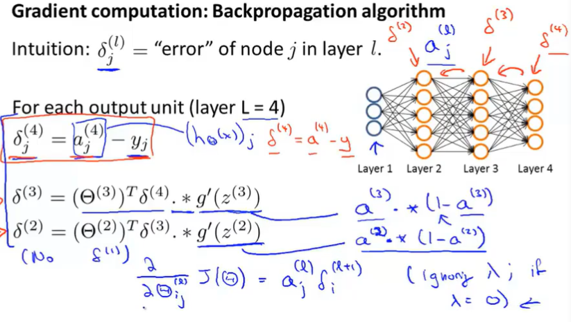
Next, in order to compute the derivatives, we’re going to use an algorithm called back propagation. The intuition of the back propagation algorithm is that for each node we’re going to compute the term $\delta ^{(l)}_j$ that’s going to somehow represent the “error” of node j in the layer l.
Recall $a ^{(l)}_j$ does the activation of the j of unit in layer l. So this $\delta$ term is in some sense going to capture our error in the activation of that neural.
$\delta ^{(4)}_j=a ^{(4)}_j-y_j$.
If you think of $\delta$$\alpha$ and y as vectors then you can take those and come up with a vectorized implementation of it.
$\delta ^{(4)}=a ^{(4)}-y$ Here, each of these is a vector whose dimension is equal to the number of output units in out network.
So we now got $\delta ^{(4)}$. What we do next is compute the delta terms for the earlier layers in our network.
Here’s a formula for computing $\delta(3)$ , $\delta^{(3)} = (\Theta ^ {(3)}) ^T\delta ^{(4)}\ast g’(z ^ {(3)})$. The term g prime of z3, that formally is actually the derivative of the activation function g evaluated at the inputs given by z3. You can get $g’(z ^{(3)}) = a ^{(3)}\ast (1-a ^{(3)})$ if put z3 in sigmoid function.
$\delta^{(2)} = (\Theta ^ {(2)}) ^T\delta ^{(3)}\ast g’(z ^ {(2)})$ $g’(z ^{(2)}) = a ^{(2)}\ast (1-a ^{(2)})$
And there is no delta 1 term, because the first layer corresponds to the input layer and that’s just the feature we observed in our training sets, so that doesn’t have any error associated with that.
The name back propagation comes from the fact that we start by computing the delta term for the output layer and then we go back a layer and compute the delta terms for the third hidden layer and then we go back another step to compute $\delta(2)$ and so, we’re sort of back propagating the errors from the output layer to layer 3 to layer 2.
Ignoring lambda or alternatively the regularization term lambda will equal to 0 $\frac{\partial}{\partial\Theta_{ij} ^{(l)}}J(\Theta)=a_{j} ^{(l)} \delta_{i} ^{l+1}$
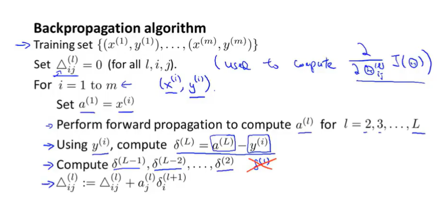
Suppose we have a training set of m examples. The first thing we’re going to do is to set these $\delta ^{(l)}_{ij}$. Triangular symbol is the capital Greek alphabet delta. $\Delta ^{(l)}_{ij}$.
The delta is to be used as accumulators that will slowly add things in order to compute these partial derivatives.
Next we’re going to loop through our training set. For the ith iteration, we’re going to working with the training example $(x ^{(i)},y ^{(i)})$.
Set $a ^{(1)} = x ^{(i)}$ and perform forward propagation to compute the activations for all layer $a ^{(l)} l=2,3,…,L$.
Next we’re going to use output label $y ^{(i)}$ to compute the term for $\delta ^{(L)}$ for the output there. $\delta ^{(i)} = a ^{(L)}-y ^{(i)}$.
Then we’re going to use the back propagation algorithm to compute $\delta ^{(L-1)},\delta ^{(L-2)},…,\delta ^{(2)}$. No delta 1 because we don’t associate an error term with the input layer.
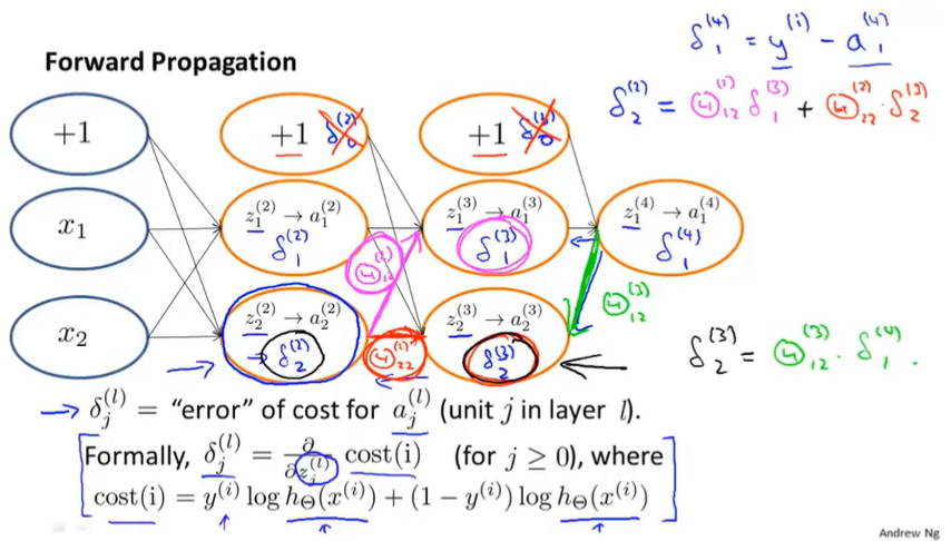
9.3 Backpropagation Intuition
Forward propagation:
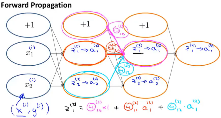
Back propagation:
One useful intuition is that back propagation is computing these $\delta ^{(l)}_j$ and we can think of these as the call error of the activation value.
9.4 Implementation Note Unrolling Parameters
Use back propagation to compute the derivatives of your cost function.
One implementation detail of unrolling parameters from matrices into vectors. Then you can pass this to an advanced authorization algorithm like fminunc for getting our for a gradient there.
|
|

9.5 Gradient Checking
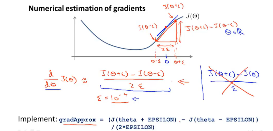
When $\Theta$ is real number
When $\Theta$ is a vector parameter
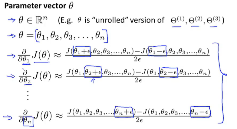
The top partial derivative of the cost function with respect to every parameter in our network. And we can then take the gradient that we got from back prop.
Check that $gradApprox\approx DVec$ If so, that implementation of back prop is correct.
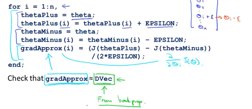
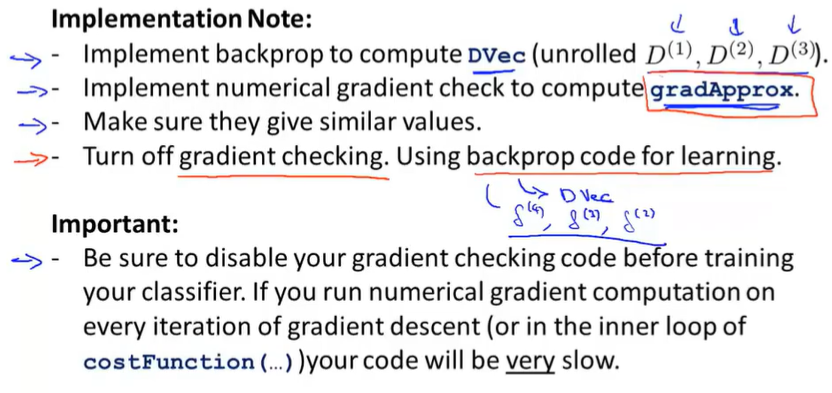
The numerical gradient checking code is a very computationally expensive, a very slow way to try to approximate the derivative. Whereas in contrast, back propagation algorithm is much more computationally efficient way of computing the derivatives. Once you’ve verified your implementation of back propagation is corrct, you should turn off gradient checking
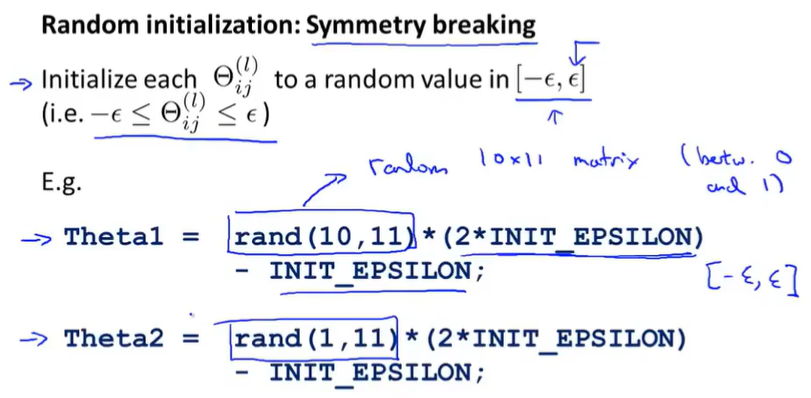
9.6 Random Initialization
If set zeros, after each update, $\Theta$ will always be same. The way to solve is to use random initialization.
9.7 Putting It Together
- Pick a network architecture(connectivity pattern between the neurons)
- Reasonable default 1 hidden layer. The more hidden units in each layer the better(slow)
Training a neural network
- Randomly initialize weights
- Implement forward propagation to get $h_\Theta(x ^{(i)})$ for any $x ^{(i)}$
- Implement code to compute cost function $J(\Theta)$
- Implement backprop to compute all partial derivatives
- Use gradient checking to compare partial derivatives computed using backpropagation and numerical estimate of gradient of $J(\Theta)$.
- Use gradient descent or advanced optimization method with backpropagation to try minimize $J(\Theta)$ as a function of parameters $\Theta$.
9.8 Autonomous Driving
10. Advice for Applying Machine Learning
10.1 Deciding What to Try Next
When you test your hypothesis on a new set of houses, you find that it makes unacceptably large errors in its predictions. What should you try next?
- Get more training examples
- Try smaller sets of features
- Try getting additional features
- Try adding polynomial features($x ^2_1,x ^2_2,x_1x_2,etc.$)
- Try decreasing $\lambda$
- Try increasing $\lambda$
In the next two videos after this, I’m going to first talk about how to evaluate learning algorithms.
In the next two videos after that, I’m going to talk about these techniques which are called the machine learning diagnostics.(A test that you can run to gain insight what is/isn’t working with a learning algorithm, and gain guidance as to how best to improve its performance.)
10.2 Evaluating a Hypothesis
The standard way to evaluate a learned hypothesis is as follows.
Split the dataset into training set and test set.
-
Typical procedure for how you would train and test the learning algorithm maybe linear regression.
- First, Learn parameter $\Theta$ from training data(minimizing training error $J(\Theta)$)
- Compute test set error.
-
Training/testing procedure for logistic regression
- Learn parameter $\Theta$ for logistic regression
- Compute test error.
- Misclassification error (0/1 misclassification error)
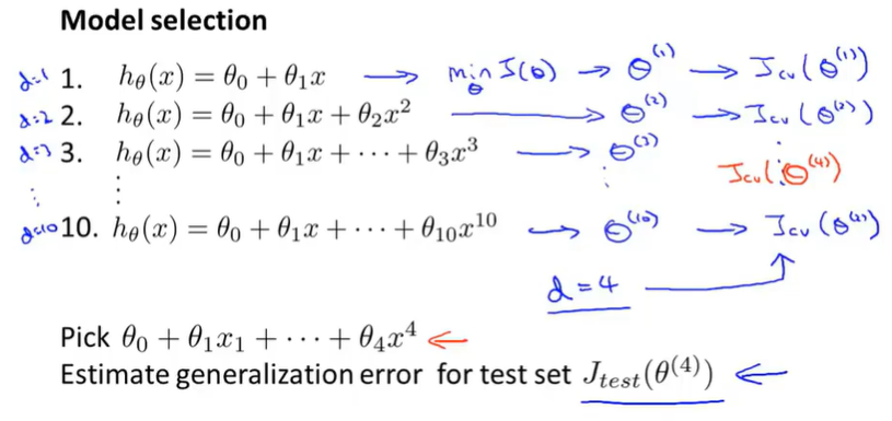
10.3 Model Selection and Train Validation Test Sets
We will see what “Switch data into train, validation and test sets. " are and how to use them to do model selection.
Model selection: choose a degree of polynomial and fit that model and also get some estimate of how well your fitted hypothesis was generalize to new examples.
Go over and get all parameters $\Theta ^1\Theta ^2…\Theta ^{10}$ , look at cross validation set error, see which model has the lowest cross validation set error.
Instead of using the test set to select the model, we’re instead going to use the validation set, or the cross validation set, to select the model.
Use the test set to measure or to estimate the generalization error of the model that was selected by the algorithm.
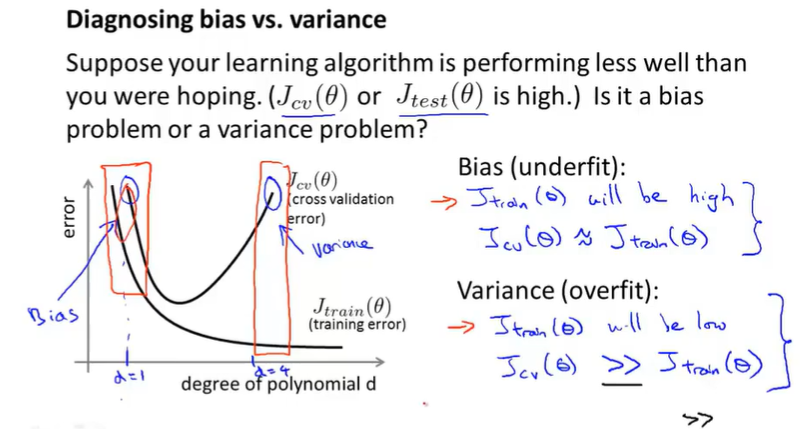
10.4 Diagnosing Bias vs. Variance
underfitting problem or an overfitting problem.
Bias(underfit): training error high cross validation error high
Variance(overfit): training error low cross validation error high
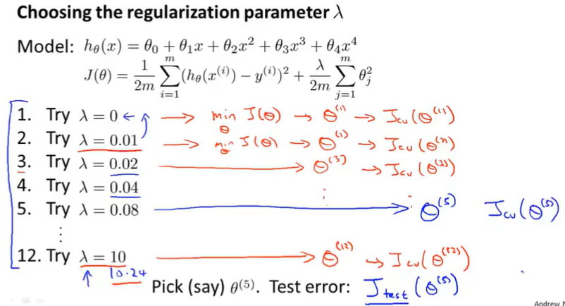
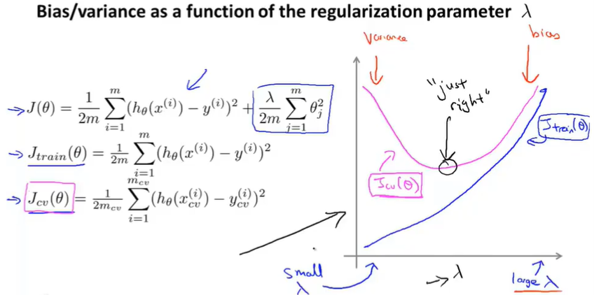
10.5 Regularization and Bias/Variance
How does regularization affect the bias ans variance of a learning algorithm?
How can we automatically choose a good value for the regularization parameter $\lambda$?
Like in model selection
- choose different $\lambda$
- minimize the cost function and get parameters vector $\Theta$
- use cross validation set to evaluate them
- choose the lowest error
- look at how well it does on the test set
You can plot $J_{train}(\Theta)$ and $J_{cv}(\Theta)$. When $\lambda$ is small it would be overfiting(variance), when $\lambda$ is large it would be lessfiting(bias).
10.6 Learning Curves
Learning curve is a useful tool that can use to diagnose if a physical learning algorithm may be suffering from bias, variance problem or a bit of both.
High bias: If a learning algorithm is suffering from high bias, getting more training data will not(by itself) help much.
High variance: If a learning algorithm is suffering from high variance, getting more training data is likely to help.
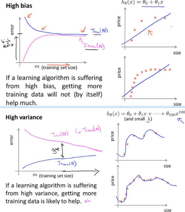
Plotting learning curves like these can often help you figure out if your learning algorithm is suffering bias, or variance or even a little bit of both.
10.7 Deciding What to Do Next (Revisited)
Our original example:
- Get more training examples——help to fix high variance
- Try smaller sets of features——help to fix high variance
- Try getting additional features——fix high bias problems
- Try adding polynomial features($x ^2_1,x ^2_2,x_1x_2,etc.$)——fix high bias problems
- Try decreasing $\lambda$——fix high bias
- Try increasing $\lambda$——fix high variance
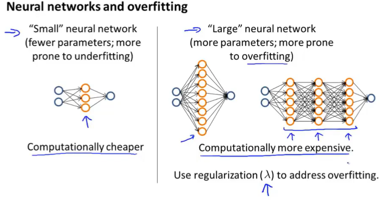
“small” neural network has few parameters and more likely to underfitting, the advantage of these small neural networks is that they are computationally cheaper.
“large” neural network with either more hidden units(a lot hidden unit in one layer) or with more hidden layers tend to have more parameters and therefore be more prone to overfitting. You can use regularization to address overfitting.
11. Machine Learning System Design
11.1 prioritizing what to work on: Spam classification example
In order to apply supervised learning, the first decision we must make is how do we want to represent x, that is the features of the email.
In practice, take most frequently occurring words ( 10,000 to 50,000) in training set, rather than manually pick 100 words.
Spend your time to make it have low error
-
Collect lots of data
- E.g. “honeypot” project.
-
Develop sophisticated features based on email routing information (from email header).
-
Develop sophisticated features for message body, e.g. should “discount” and “discounts” be treated as the same word? How about “deal” and “Dealer”? Features about punctuation?
-
Develop sophisticated algorithm to detect misspellings (e.g. m0rtgage, med1cine, w4tches.)
11.2 Error Analysis
11.3 Error Metrics for Skewed Classes
If the number of positive examples is much smaller than the number of negative examples, we call it the case of skewed classes.
Facing this problem, we want to come up with a different error metric or a different evaluation metric. One such evaluation metric are what’s called precision/recall.
| 1 | 0 | ←Actual clss | |
|---|---|---|---|
| 1 | True Positive(TP) | False Positive(FP) | Precision |
| 0 | False Negative(FN) | True Negative(TN) | |
| ↑Predicted class | Recall |
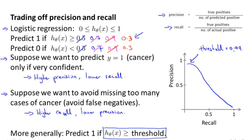
precision: TP/predicted positives = TP/(TP+FP)
recall: TP/actual positives = TP/(TP+FN)
11.4 Trading Off Precision and Recall
For many applications, we’ll want to somehow control the trade off between precision and recall.
If you predict y=1 only if very confident by increase threshold, there will be higher precision and lower recall
If you avoid missing too many cases of cancer(FN) by decreasing threshold, there will be higher recall and lower precision
Average: $\frac{P+R}2$ is not a good method to evaluate
Fscore: $2\frac{PR}{P+R}$ is a better way
11.5 Data For Machine Learning
12. Support Vector Machines
SVM, compared with LR and NN, sometimes gives a cleaner and more powerful way of learning complex nonlinear functions.
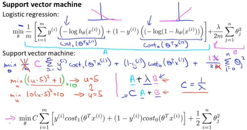
12.1 Optimization Objective
replace(simplify) the cost function of LR and make it easier to calculate
Cost function:
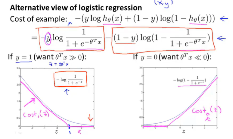
Finally unlike LR, the SVM doesn’t output the probability. Instead what we have is this cost function, which we minimize to get parameters $\theta$. And what SVM does is just makes a prediction of y being equal 1 or 0 directly.
12.2 Large Margin Intuition
Cost function:
if y=1, we want $\Theta^Tx>=1$(not just >= 0)
if y=0, we want $\Theta^Tx<=-1$(not just < 0)
This builds in an extra safety factor or safety margin factor into the SVM.
Let’s see what happens or what the consequences of this are in the context of the SVM.
If C is very large, what we need to do is make first term equal to 0.
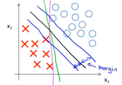
It turns out that when you solve this optimization problem, when you minimize this as a function of the parameters $\Theta$, you get a very interesting decision boundary.
In linearly separable case, the black line is a much better decision boundary than others. mathematically, this line has large distance. That distance is called the margin.
C like $\lambda$
If C is very large the decision boundary will be sensible to few outliers.
If C is not too large, SVM also do fine and reasonable things even your data is not linearly separable.
12.3 Mathematics Behind Large Margin Classification(optional)
Math behind large margin classification
$u = \begin{bmatrix}u_1 \\ u_2\end{bmatrix} v=\begin{bmatrix}v_1 \\ v_2\end{bmatrix}$
Inner product = $u^Tv = u_1v_1+u_2v_2$
$|u| = \sqrt{u ^2_1+u ^2_2}$
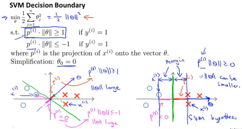
Optimization objective = $\frac12(\Theta ^2_1+\Theta ^2_2) = \frac12(\sqrt{\Theta ^2_1+\Theta ^2_2}) ^2 = \frac12|\Theta| ^2$
s.t. $\Theta ^Tx ^{(i)}>=1$ if $y ^{(i)}=1$
$\Theta ^Tx ^{(i)}<=-1$ if $y ^{(i)}=0$
so $\Theta ^Tx ^{(i)} = \Theta_1x ^{i}_1+\Theta_2x ^{(i)}_2$
The decision boundary and parameters $\Theta$ are 90 degree orthogonal, we need a small range of parameters $\Theta$, that mean only when $p^{(i)}$ is big not small, that meet the condition $p^{(i)}\cdot{\left| \theta \right|}$ >= 1 or <= -1 since $|\Theta|$ is always positive.
The magnitude of the margin is exactly the values of $p ^{(1)}p ^{(2)}p ^{(3)}$ and so on. By making the margin large, SVM can end up with a smaller value for the norm of $\Theta$, which is what it is trying to do in the objective. And this is why SVM ends up with a large margin classifiers, because it is trying to maximize the norm of these $p ^{(i)}$ which is the distance from the training examples to the decision boundary.
12.4 Kernels I
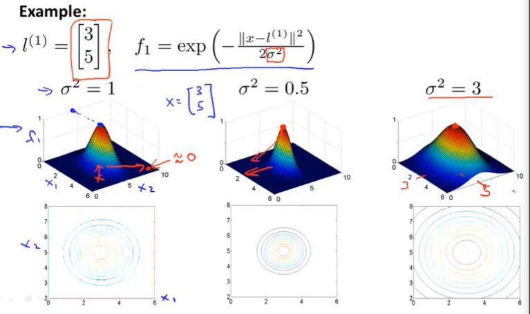
$f_1=similarity(x,l ^{(1)})=e(-\frac{|x-l ^{(1)}| ^2}{2\sigma ^2})$
$f_2=similarity(x,l ^{(2)})=e(-\frac{|x-l ^{(2)}| ^2}{2\sigma ^2})$
$f_3=similarity(x,l ^{(3)})=e(-\frac{|x-l ^{(3)}| ^2}{2\sigma ^2})$
These particular choice of similarity function is called Gaussian kernel. But the way the terminology goes is that, in the abstract these different similarity functions are called kernels and we can have different similarity functions and the specific example I’m giving here is called Gaussian kernel.
$If x\approx l ^{(1)} Then f_1 \approx e ^{-0} \approx 1$
If x is far from $l ^{(1)}$ Then $f_1=e ^{\text{-large number} } \approx 0$
We predict 1 when $θ_0+θ_1f_1+θ_2f_2+θ_1f_3>=0$
Let $\Theta_0=-0.5 \Theta_1=\Theta_2=1 \Theta_3=0$, and we can judge whether the point positive or not.
For the purple point $f1=1 f2=0 f3=0$ so $θ_0+θ_1f_1+θ_2f_2+θ_1f_3 = -0.5+1 = 0.5 > 0$ . So this point is positive.
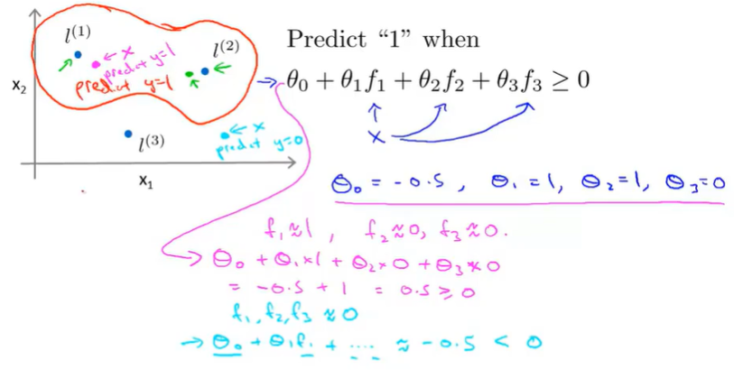
This is how with the definition of the landmarks and of the kernel function we can learn pretty complex non-linear decision boundary.
12.5 Kernels II
Throw in some of the missing details and also, say a few words about how to use these ideas in practice. Such as, how to pertain to the bias variance trade-off in SVM.
Where to get landmarks $l ^{(1)}l ^{(2)}l ^{(3)}$? The idea here is we’re gonna take the examples and for every training example, we are just put landmarks as exactly the same locations as the training examples.
Given an example x we are going to compute features as $f_1 f_2$ and so on. And these then give me a feature vector. $f = \begin{bmatrix}f_1 \\ f_2 \\ … \\ f_m \end{bmatrix}$ By convention, we can add an $f_0=1$
How to choose SVM parameters?:
C(=$\frac1\lambda$) Large C: Lower bias, high variance.
Small C: Higher bias, low variance.
$\sigma ^2$ in Gaussian kernel: Large $\sigma ^2$, features f vary more smoothly, higher bias, lower variance.
Small $\sigma ^2$: features f vary less smoothly. lower bias, higher variance.
12.6 Using An SVM
kernel:
- No kernel(“linear kernel”) predict “y=1” if $\Theta ^Tx>=0$(when n large and m small)
- Gaussian kernel(when n small m large non-linear boundary) [Note: Do perform feature scaling before using Gaussian kernel]
- Polynomial Kernel
- String kernel
- chi-square kernel
- histogram intersection kernel
Multiclass classification:
Many SVM packages already have built-in multi-class classification functionality.
Otherwise, use one-vs.-all method. (Train K SVMs, one to distinguish y=i from the rest, for i=1,2…k), get $\Theta ^{(1)}\Theta ^{(2)}…\Theta ^{(K)}$ Pick class i with largest ${\Theta ^{(i)}} ^Tx$.
LR vs. SVM:
If n is large(relative to m) use LR or SVM without a kernel(“linear kernel”)
If n is small, m is intermediate: use SVM with Gaussian kernel
If n is small, m is large: create/add more features, then use LR or SVM without a kernel
Neural network likely to work well for most if these settings, but may be slower to train.
13. Clustering
13.1 Unsupervised Learning——Introduction
Our first unsupervised learning where we learn unlabeled data instead of labeled data.
13.2 K-Means Algorithm
K-Means Algorithm by far the most popular most widely used clustering algorithm.
Input:
- K(number of clusters)
- Training Set{$x ^{(1)} x ^{(2)},…x ^{(m)}$}
STEP:
Randomly initialize K cluster centroids $\mu_1\mu_2…\mu_K$
Repeat:{
for i 1 to m: $c ^{(i)} = $index(for 1 to K) of cluster centroid closest to $x ^{(i)}$ [cluster assignment step]
for k = 1 to K: $\mu_k$ = average(mean) of points assigned to cluster k [move centroid step]
}
K-means for non-separated clusters
Like T-shirt sizing problem. You have many body shape and you need to decide how much clusters you need like S,M,L,XL. Then use algorithm to separate them.
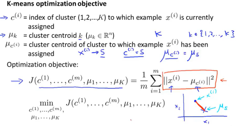
13.3 Optimization Objective
$\mu_{c ^{(i)} }$ = cluster centroid of cluster to which example $x ^{(i)}$ has been assigned
$x ^{(i)}$ is the training point , we want to minimize the sum of distance between points and cluster centroid
13.4 Random Initialization
Randomly pick K training examples.
Set $\mu_1,…\mu_k$ equal to these K examples.
Local optima:
initialize K-means lots of times and run K-means lots of times
for ( initialize, run K-means ,compute cost function)
pick clustering that gave lowest cost
13.5 Choosing the Number of Clusters
Elbow method:
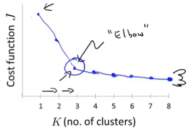
Sometimes, you’re running K-means to get clusters to use for some later/downstream purpose. Evaluate K=means based on a metric for how well it performs for that later purpose.
14. Dimensionality Reduction
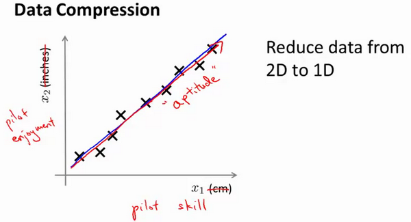
14.1 Motivation I—— Data Compression
Reduce data from 2D to 1D:
Reduce data from 3D to 2D:
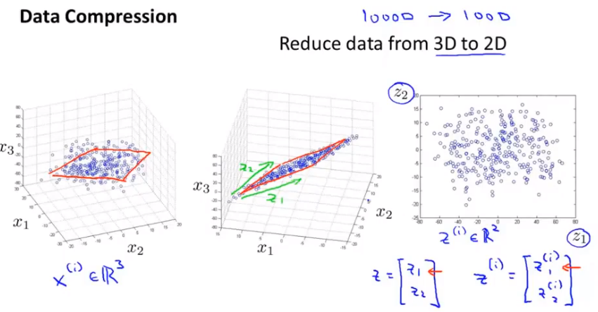
All these data maybe all of this data maybe lies roughly on the plane. And what we can do with dimensionality reduction is take all of this data and project the data down onto a two dimensional plane.
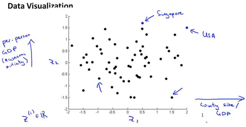
14.2 Motivation II——Visualization
Application of dimensionality reduction——visualize the data. For a lot of machine learning applications, it helps us to develop effective learning algorithms. if we can understand our data better, there is some way of visualizing the data better, and so, dimensionality reduction offers us another useful tool to do so.
If we can use z1 an z2 to summarizes 50 numbers, then plot these countries in R2 and the understand this sort of features of different countries will be better. What you can do is reduce the data from 50D to 2D. z1 and z2 doesn’t astride a physical meaning.
14.3 Principal Component Analysis Problem Formulation
Let try to formulate precisely exactly what we would like PCA to do.
PCA tries to find a lower-dimensional surface onto which to project the data.
Reduce from 2D to 1D: find a direction onto thich to project the data so as to minimize the projection error.
Reduce from nD to kD: find k vectors onto which to project the data so as to minimize the projection error. (3D to 2D together vectors define a plain or 2D surface)
PCA&LR
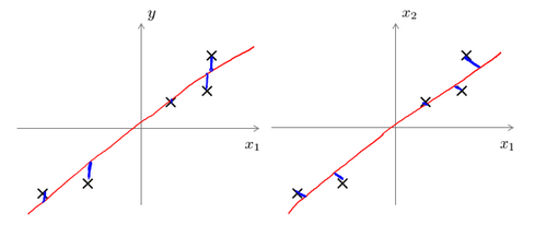
LR fitting a straight line so as to minimize the squared error between a point and the straight line. Notice we drawing distance vertically(point and the point on the line). PCA tries to minimize the shortest orthogonal distances( point and line)
14.4 Principal Component Analysis Algorithm
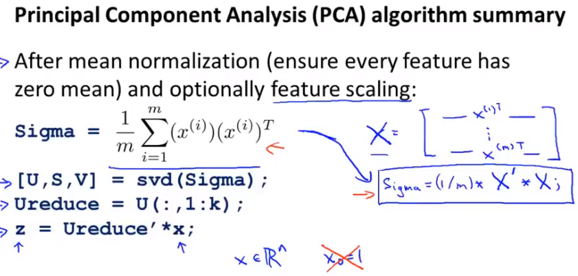
Before applying PCA, there is a data pre-processing step which you should always do.
Preprocessing(features scaling/mean normalization): First compute the mean of each feature $\mu_j = \frac1m\sum ^m_{i=1}x_j ^{(i)}$ and replace each feature $x_j = x_j-\mu_j$.
Compute covariance matrix: $\Sigma = \frac1m\sum ^n_{i=1}(x ^{(i)})(x ^{(i)}) ^T$
Compute eigenvectors: [U,S,V] = svd(Sigma) [svd:singular value decomposition]
S is a Diagonal matrix.
U is a NxN dimensional vector, reduce to k dimensional vector
$z ^{(i)}=U ^T_{reduce}*x ^{(i)}$
14.5 Choosing The Number Of Principal Components
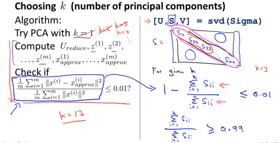
Choosing k(number of principle components)
Average squared projection error:
Total variation in the data:
Typically, choose k to be smallest value so that
$\frac{\text{Average squared projection error} } {\text{Total variation in the data} }<=0.01$ (99% of variance is retained)
Run SVD once and you get Diagonal matrix, then calculate k.
$\frac {\Sigma ^k_{i=1}s_{ii} }{\Sigma ^n_{i=1}s_{ii}}\geq0.99$
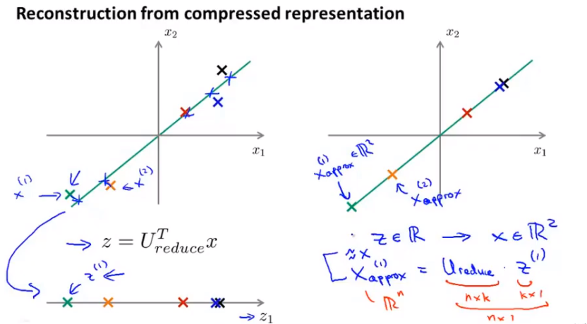
14.6 Reconstruction from Compressed Representation
14.7 Advice for Applying PCA
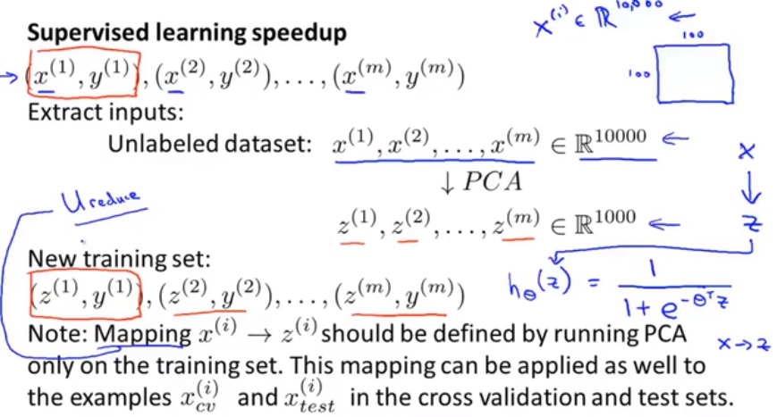
Speedup supervised learning:
100x100 pictures
- Apply PCA and reduce to 1000 dimensional features vectors.
- Feed new training set to a learning algorithm.
- For example X, map it through the same mapping that was found by PCA to get corresponding Z and fed to hypothesis and make a prediction.
Application of PCA
- Compression(Choose K by percentage of variance retained)
- Reduce memory/disk needed to store data
- Speed up learning algorithm
- Visualization(k=2 or k=3)
Bad use of PCA: To prevent over-fitting
Use $z ^{(i)}$ instead of $x ^{(i)}$ to reduce the number of features to k < n. (fewer features, less likely to over-fit). Actually isn’t a good way to address over-fitting. Use regularization instead. Why? PCA throws away some information, reduce dimension of your data without knowing what the values of y is. It might also throw away some valuable information. Use regularization will often gives you at least as good a method for preventing over-fitting.
Often at very start of a project, someone will just write out a project plan and use PCA inside. How about doing the whole thing without using PCA? Before implementing PCA, first try running whatever you want to do with original/raw data $x ^{(i)}$. Only if that doesn’t do what you want, then implement PCA and consider using $z ^{(i)}$.
15. Anomaly Detection
Anomaly Detection is mainly for unsupervised problem, that there’s some aspects of it that are also very similar to sort of the supervised learning problem.
15.1 Problem Motivation
Density estimation:
dataset: {$x ^{(1)},x ^{(2)},x ^{(3)},….x ^{(m)}$}
$if \quad p(x) \begin{cases} < \varepsilon & anomaly \\ > =\varepsilon & normal \end{cases}$
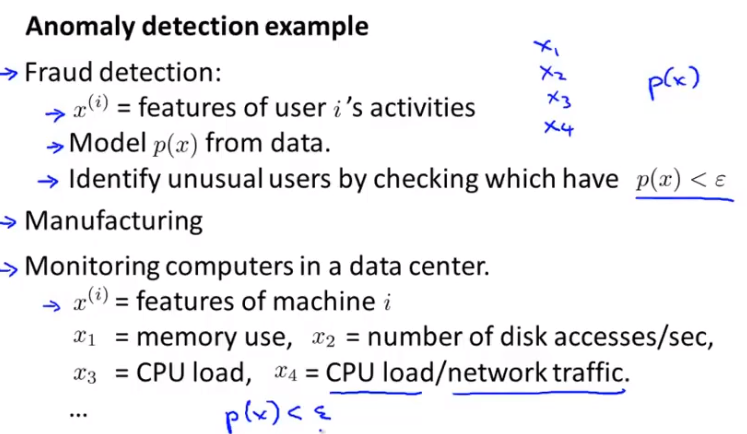
Anomaly detection example:
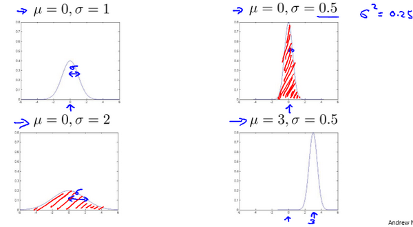
15.2 Gaussian Distribution
Gaussian distribution = Normal distribution
$x \sim N(\mu, \sigma ^2)$
$p(x,\mu,\sigma ^2)=\frac{1}{\sqrt{2\pi}\sigma}\exp\left(-\frac{(x-\mu) ^2}{2\sigma ^2}\right)$
$\mu=\frac{1}{m}\sum\limits_{i=1} ^{m}x ^{(i)}$
$\sigma ^2=\frac{1}{m}\sum\limits_{i=1} ^{m}(x ^{(i)}-\mu) ^2$
15.3 Algorithm
Apply Gaussian distribution to develop an anomaly detection algorithm.
Given dataset $x ^{(1)},x ^{(2)},…,x ^{(m)}$, which is distributed according to a Gaussian distribution. So $\mu_j=\frac1m\sum\limits_{i=1} ^mx_j ^{(i)}$ and $\sigma_j ^2=\frac1m\sum\limits_{i=1} ^m(x_j ^{(i)}-\mu_j) ^2$. These data may be vectorized versions.
Compute p(x).
$p(x)=\prod\limits_{j=1} ^np(x_j;\mu_j,\sigma_j ^2)=\prod\limits_{j=1} ^1\frac{1}{\sqrt{2\pi}\sigma_j}exp(-\frac{(x_j-\mu_j) ^2}{2\sigma_j ^2})$. It is anomaly if $p(x) < \epsilon$.
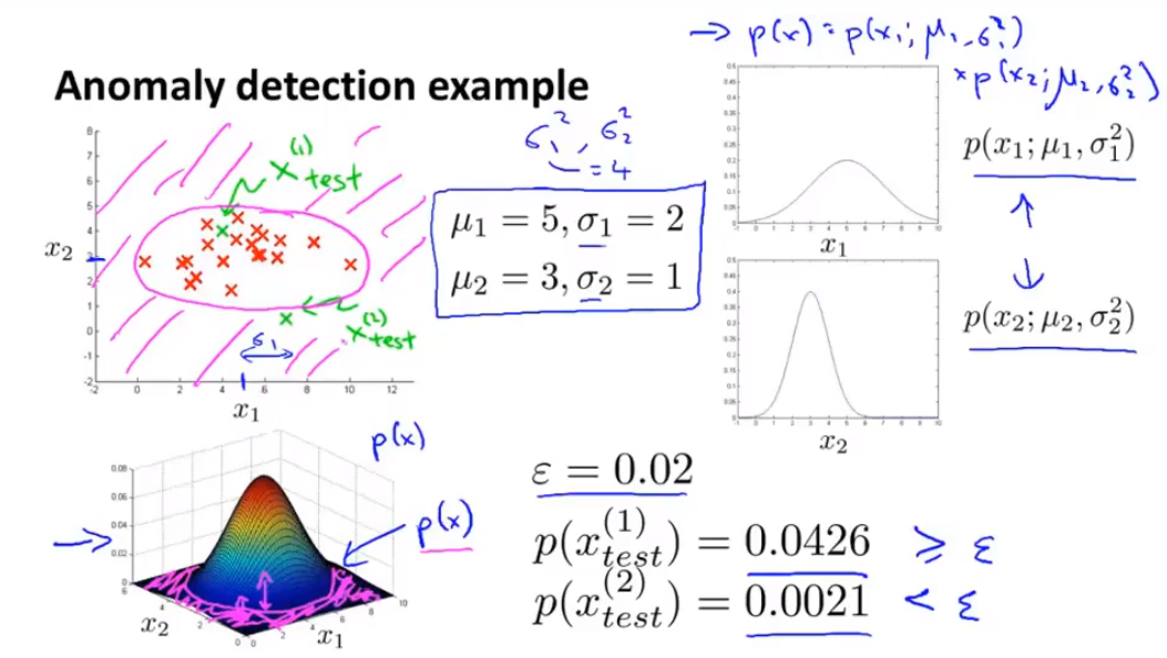
The height of this 3-D surface is p(x). To check a point is anomaly or not, we set some very small value for epsilon, and then compute p(x) of the point. If p(x) greater than or equal to epsilon, then we think it is not an anomaly. But if p(x) is smaller then epsilon, that is indeed an anomaly.
15.4 Developing and Evaluating an Anomaly Detection System
How to develop a specific anomaly detection algorithm
How to evaluate an anomaly detection algorithm
Assume we have some labeled data, of anomalous and non-anomalous examples.
And we are going to define a cross validation set and a test set, with which to evaluate a particular anomaly detection algorithm.
Example:
10000 good engines and 20 flawed engines
Training set: 6000 good engines
CV: 2000 good engines(y=0) 10 anomalous(y=1)
Test: 2000 good engines(y=0) 10 anomalous(y=1)
Get training set and fit p(x)
Evaluate: It is a very skewed data set, then predicting y equals 0 all the time will have very high classification accuracy. Instead, we should use evaluation metrics like computing the Precision/Recall or do things like compute the F1 score, which is a single real-number way of summarizing the precision and the recall numbers.
Use cross validation set to choose parameter $\epsilon$ which maximizes F1 score or the otherwise does well on your cross validation sets.
15.5 Anomaly Detection vs. Supervised Learning
If we have this labeled data, we have some examples that are known to be anomalies and some that are known not to be not anomalies, why don’t we just use a supervised learning algorithm, so why don’t we just use logistic regression or a neural network to try to learn directly from our labeled data, to predict whether y equals one or y equals zero?
| Anomaly Detection | Supervised Learning |
|---|---|
| Very small number of positive examples. Large number of negative examples. | Large number of positive and negative examples simultaneously. |
| Many different “types” of anomalies. Hard for any algorithm to learn from positive examples what the anomalies look like. | Enough positive examples for algorithm to get a sense of what positive examples are like. |
| Future anomalies mat look nothing like any of the anomalous examples we’ve seen so far. | Future positive examples likely to be similar to ones in training set. |
| Examples: Fraud detection, Manufacturing(aircraft engines), Monitoring machines in a data center | Examples: Email spam problem, Weather prediction, Cancer classification |
15.6 Choosing What Features to Use
You have seen the anomaly detection algorithm and we’ve talked about how to evaluate an anomaly detection algorithm.
It turns out that when you’re applying anomaly detection, one of the things that has a huge effect on how well it does, is what features you use, and what features you choose, to give the anomaly detection algorithm.
Transformations of the data in order to make it look more Gaussian might work a bit better.
We can use log function($x = log(x+c), c>=0$) to transform the data, function in python np.log1p = log(x+1)
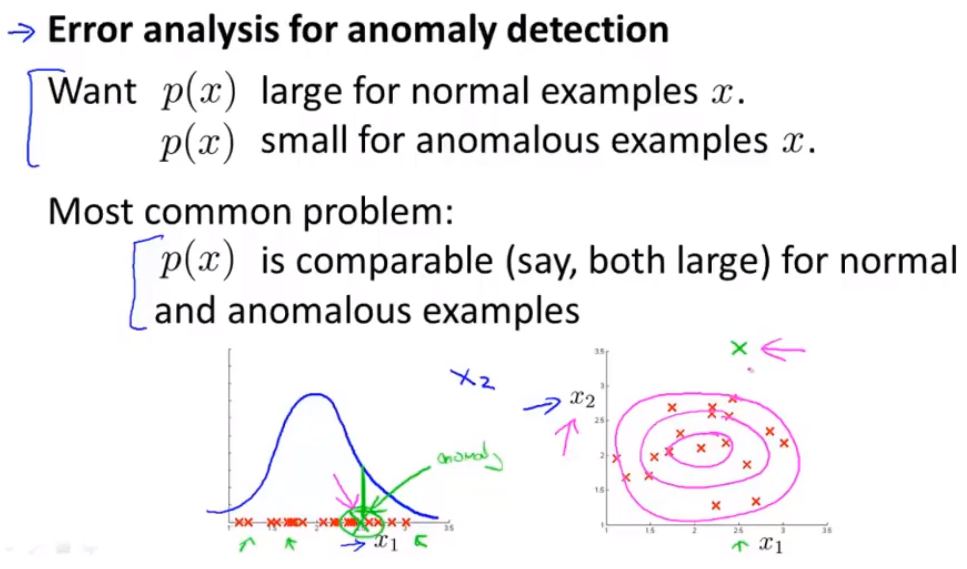
Error analysis for anomaly detection
run on CV and look at the examples it gets wrong and come up with extra features to help algorithm.
Monitoring computers in a data center
Choose features that might take on unusually large or small values on the event of an anomaly.
$x_1$ = memory use of computer
$x_2$ = number of disk accesses/sec
$x_3$ = CPU load
$x_4$ = network traffic
to check infinite loop, we may need a new feature $x_5 = \frac{x_3}{x_4}$. this may take on a unusually large value if one of the machines has a very large CPU load but not that much network traffic. So that will help your anomaly detection capture, a certain type of anomaly.
15.7 Multivariate Gaussian Distribution (Optional)
15.8 Anomaly Detection using the Multivariate Gaussian Distribution (Optional)
16. Recommender Systems
16.1 Problem Formulation
Recommender systems is an important application of machine learning.
Through recommender systems, will be able to go a little bit into this idea of learning the features.
Recommender systems look at what books you may have purchased in the past, or what movies you have rated.
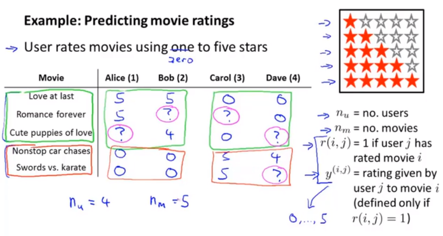
And so, our job in developing a recommender system is to come up with a learning algorithm that can automatically go fill in these missing values.
16.2 Content Based Recommendations
If we have features like these then each movie can be represented with a feature vector.
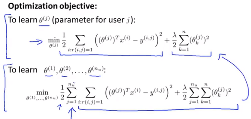
We could treat predicting the ratings of each user as a separate linear regression problem.
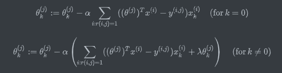
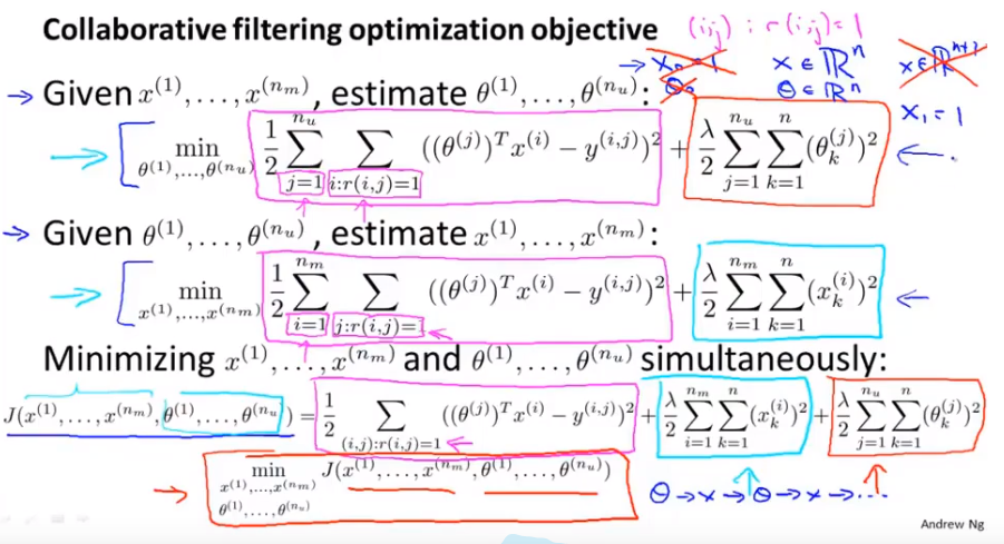
For each user j, learn a parameter $\Theta ^{(j)} \in \mathbb{R} ^3$. Predict user j as rating movie i with $(\Theta ^{(j)} ) ^Tx ^{(i)}$ stars.
16.3 Collaborative Filtering
we’re talking a recommender system that’s called collaborative filtering, which start to learn for itself what features to use.
Know $\Theta$ in advance, we can get the features X since $(\Theta ^{(j)} ) ^Tx ^{(i)} = movie ratings$.
16.4 Collaborative Filtering Algorithm
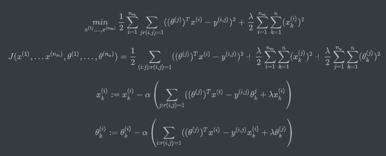
- Initialize $x ^{(1)}…x ^{(n_m)},\Theta ^{(1)}…\Theta ^{(n_m)}$ to small random values.
- Minimize $J(x ^{(1)}…x ^{(n_m)},\Theta ^{(1)}…\Theta ^{(n_m)})$ using gradient descent(or an advanced optimization algorithm).
- For a user with parameters $\Theta$ and a movie with(learned) features x, predict a star rating of $\Theta ^Tx$.
16.5 Vectorization——Low Rank Matrix Factorization
Like matrix multiplication
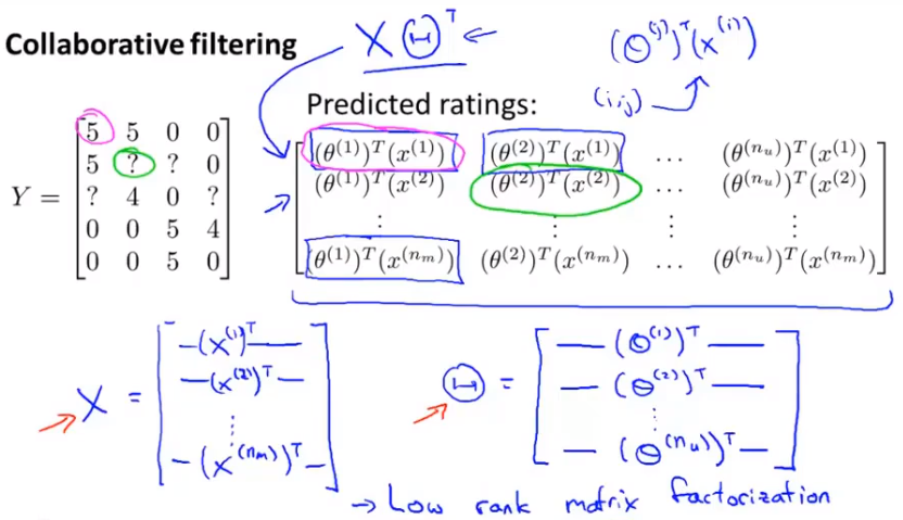
Finding related movies:
For each product i, we learn a feature vector $x ^{(i)}$.
small $|x ^{(i)}-x ^{(j)}|$ ——> movie j and movie i are “similar”.
16.6 Implementation Detail——Mean Normalization
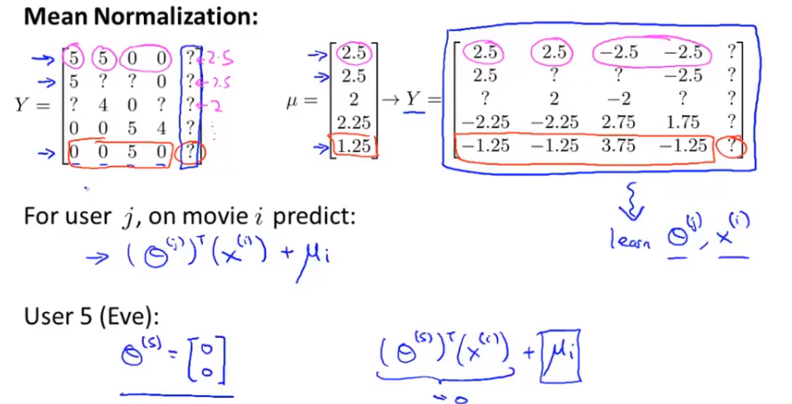
If user Eve hasn’t rated any movies. The only Influential part is the last part. We want to choose vector theta 5 so that the last regularization term is as small as possible. We would end up getting a $\Theta$ that is all 0.
The idea of mean normalization will let us fix this problem.
I’m going to compute the average rating($\mu$) that each movie obtained. All the movie ratings subtract off the mean rating.
So, what I’m doing is just normalizing each movie to have an average rating of zero.
Now use this set of ratings with my collaborative filtering algorithm. Our last prediction should be $(\theta ^{(j)})^T x ^{(i)}+\mu_i$. This mean user Eve will get the average rating.
17. Large Scale Machine Learning
17.1 Learning With Large Datasets
Before investing the effort into actually developing and the software needed to train these massive models is often a good sanity check, if training on just a thousand examples might do just as well.
If we have a high variance model, we may need large datasets.
If we have a high bias model, large datasets may don’t help.
So in large-scale machine learning, we like to come up with computationally reasonable ways, or computationally efficient ways, to deal with very big data sets.
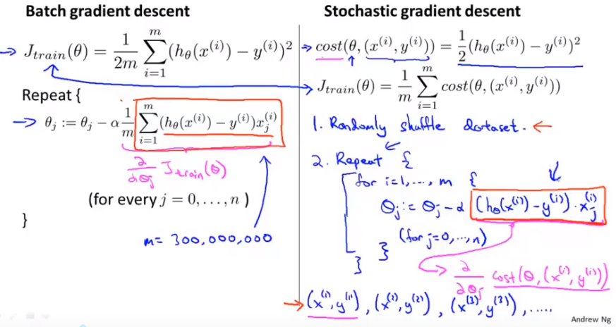
17.2 Stochastic Gradient Descent
we’ll talk about a modification to the basic gradient descent algorithm called Stochastic gradient descent, which will allow us to scale these algorithms to much bigger training sets.
If dataset is large, it’s gonna take a long time in order to get the algorithm to converge.(Batch gradient descent)
In contrast to Batch gradient descent, what we are going to do is come up with a different algorithm that doesn’t need to look at all the training examples in every single iteration, but that needs to look at only a single training example in one iteration.(Stochastic gradient descent)
17.3 Mini-Batch Gradient Descent
Batch gradient descent: Use all m examples in each iteration
Stochastic gradient descent: Use 1 example in each iteration
Mini-batch gradient descent: Use b examples in each iteration
b = mini-batch size usually b=10(2-100)
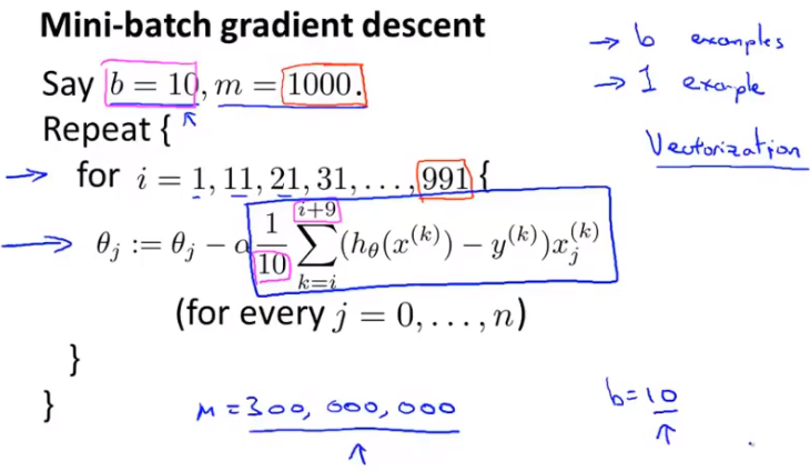
Why do we want to look at b examples at a time rather than look at just a single example at a time as the Stochastic gradient descent?
The answer is in vectorization.
Mini-batch gradient descent is likely to outperform Stochastic gradient descent only if you have a good vectorized implementation. In that case, the sum over 10 examples can be performed in a more vectorized way which will allow you to partially parallelize your computation over the ten examples.
17.4 Stochastic Gradient Descent Convergence
By using a smaller learning rate, you’ll end up with smaller oscillations.
To get a smoother curve, you need to increase the number of examples.
When curve looks like it’s increasing, what you really should do is use a smaller value of the learning rate alpha.
If you want stochastic gradient descent to actually converge to the global minimum, there’s one thing which you can do which is you can slowly decrease the learning rate alpha over time.$\alpha = \frac{const1}{iterationNumber + const2}$
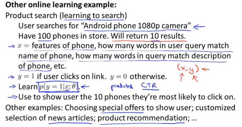
17.5 Online Learning
For a continuous stream of data from online website.
When a user come in the website, we get a example (x,y) and learn from that and discard it.
This sort of online learning algorithm can also adapt to changing user preferences and kind of keep track of what your changing population of users may be willing to pay for.
The problem of learning the predicted click-through rate, the predicted CTR.
17.6 Map Reduce and Data Parallelism
Assign tasks to multiple computers on average then centralized master server combine results together.
On a single multi-core computer, you can split the training sets into pieces and send the training set to different cores within a single box.
we talked about the MapReduce approach to parallelizing machine learning by taking a data and spreading them across many computers in the data center. Although these ideas are critical to parallelizing across multiple cores within a single computer as well.
18. Application Example: Photo OCR
18.1 Problem Description and Pipeline
Photo OCR stands for Photo Optical Character Recognition. The photo OCR problem focuses on how to get computers to read the text to the purest in images that we take.
First, given the picture it has to look through the image and detect where there is text in the picture.
Read the text in those regions.
Doing OCR from photographs today is still a very difficult machine learning problem.
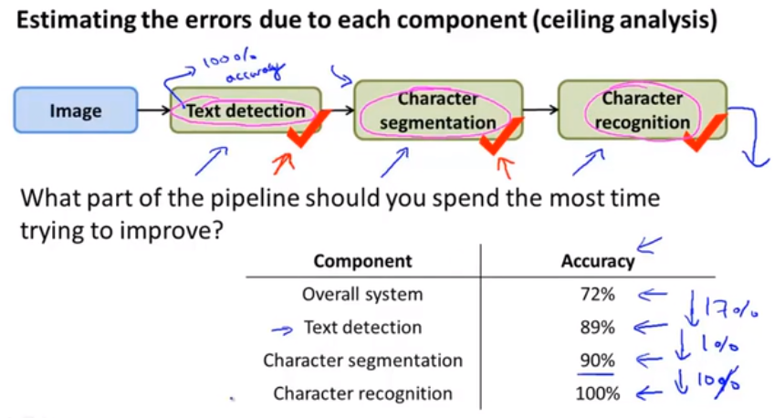
Photo OCR pipeline:
- Text detection
- Character segmentation
- Character classification

18.2 Sliding Windows
Pedestrian detection:
Supervised learning for pedestrian detection(sliding windows classifier)
shift the rectangle over each time is a parameter called the step size(also called the slide parameter)
we can choose a big rectangle and resize to the smaller one and get it detected by classifier.
Text detection:
- use classifier to get the possibility of text
- apply expansion operator and expand white pixel
- rule out strange rectangles and draw rectangles around text
How do we segment out the individual characters in this image?
use a supervised learning to decide if there is split between two characters
18.3 Getting Lots of Data and Artificial Data
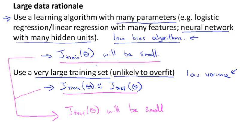
One of the most reliable ways to get a high performance machine learning system is to take a low bias learning algorithm and to train it on a massive training set. But where did you get so much training data from?
Artificial data synthesis [creating new data from scratch, amplify that training set or turn to a large one]
Create new: downloaded font
Amplify: artificial stretching or artificial distortions
Discussion on getting more data:
- Make sure you have a low bias classifier before expending the effort. (Plot learning curves). E.g. keep increasing the number of features/number of hidden units in neural network until you have a low bias classifier.
- “How much work would it be to get 10x as much data as we currently have?”
- Artificial data synthesis
- Collect/label it yourself
- Crowd source(E.g. Amazon Mechanical Turk)
18.4 Ceiling Analysis——What Part of the Pipeline to Work on Next
-
go to my test set and just give it the correct answers for the text detection part of the pipeline.
-
And now going to give the correct text detection output and give the correct character segmentation outputs and manually label the correct segment orientations of text into individual characters.
Now, the nice thing about having done this analysis analysis is we can now understand what is the upside potential for improving each of these components.
text detection——17 percent performance gain
character segmentation——1 percent performance gain
character recognition——10 percent performance gain
ceiling analysis gives the upside potential